Three-Body Problem

Problem Definition

In this problem, we consider the circular restricted three body problem in which a spacecraft evolves under the influence of the Earth and the Moon. The second order nondimensional equations of motion of this problem are

$$\ddot{x}-2\dot{y}-x = -\frac{(1-\mu)(x+\mu)}{d^3}-\frac{\mu(x-1+\mu)}{r^3}$$

$$\ddot{y}+2\dot{x}-y = -\frac{(1-\mu)y}{d^3}-\frac{\mu y}{r^3}$$

$$\ddot{z} = -\frac{(1-\mu)z}{d^3}-\frac{\mu z}{r^3}$$

where

$$d=\left[(x+\mu)^2+y^2+z^2\right]^{\frac{1}{2}}$$

$$r=\left[(x-1+\mu)^2+y^2+z^2\right]$$

$\mu$ is a parameter of the system. For the Earth-Moon system, $\mu=0.0123$. Rewriting this system in state space form yields

$$\dot{x}_1=x_4$$

$$\dot{x}_2=x_5$$

$$\dot{x}_3=x_6$$

$$\dot{x}_4=x_1+2x_5-\frac{(1-\mu)(x_1+\mu)}{d^3}-\frac{\mu(x_1-1+\mu)}{r^3}$$

$$\dot{x}_5=-2x_4+x_2-\frac{(1-\mu)x_2}{d^3}-\frac{\mu x_2}{r^3}$$

$$\dot{x}_5=-\frac{(1-\mu)x_3}{d^3}-\frac{\mu x_3}{r^3}$$

Implementation

The problem is solved using Dop853. The crate is first imported and the modules are brought into scope:

use ode_solvers::dop853::*;
use ode_solvers::*;

Type aliases are then defined for the state vector and the time:

type State = Vector6<f64>;
type Time = f64;

Next, we define the problem specific structure which will contain a single parameter:

struct ThreeBodyProblem {
  mu: f64,
}

for which we implement the System<V> trait:

impl ode_solvers::System<State> for ThreeBodyProblem {
    fn system(&self, _t: Time, y: &State, dy: &mut State) {
        let d = ((y[0] + self.mu).powi(2) + y[1].powi(2) + y[2].powi(2)).sqrt();
        let r = ((y[0] - 1.0 + self.mu).powi(2) + y[1].powi(2) + y[2].powi(2)).sqrt();

        dy[0] = y[3];
        dy[1] = y[4];
        dy[2] = y[5];
        dy[3] = y[0] + 2.0 * y[4]
            - (1.0 - self.mu) * (y[0] + self.mu) / d.powi(3)
            - self.mu * (y[0] - 1.0 + self.mu) / r.powi(3);
        dy[4] = -2.0 * y[3] + y[1] - (1.0 - self.mu) * y[1] / d.powi(3) - self.mu * y[1] / r.powi(3);
        dy[5] = -(1.0 - self.mu) * y[2] / d.powi(3) - self.mu * y[2] / r.powi(3);
    }
}

The system is created together with the intial state vector of the spacecraft in the main function. A Dop853 structure is created and the integrate() function is called. The result is handled with a match statement.

fn main() {
    let system = ThreeBodyProblem {mu: 0.012300118882173};

    let y0 = State::new(-0.271, -0.42, 0.0, 0.3, -1.0, 0.0);

    let mut stepper = Dop853::new(system, 0.0, 150.0, 0.001, y0, 1.0e-14, 1.0e-14);
    let res = stepper.integrate();

    // Handle result
    match res {
        Ok(stats) => {
            stats.print();
            // Do something with the results...
            // let path = Path::new("./outputs/three_body_dop853.dat");
            // save(stepper.x_out(), stepper.y_out(), path);  
            // println!("Results saved in: {:?}", path);
        },
        Err(_) => println!("An error occured."),
    }
}

Results

The trajectory of the spacecraft for a duration of 150 (dimensionless time) is shown on the following figure:

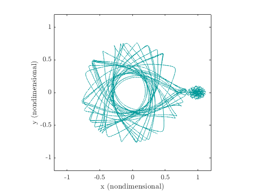
On that figure, the Earth is located at (0, 0) and the Moon is at (0.9877, 0). We see that the spacecraft is first on an orbit about the Earth before moving to the vicinity of the Moon. The accuracy of the integration can be assessed by looking at the Jacobi constant. The Jacobi constant is given by

$$C=\frac{2(1-\mu)}{d} + \frac{2\mu}{r} + x^2 +y^2 - v^2$$

and is an integral of the motion (i.e. is constant as long as no external force is applied). Based on the initial conditions, the Jacobi constant yields

$$C_0=3.1830$$

By computing the Jacobi constant at each time step and plotting the difference $C-C_0$, we get the figure below:

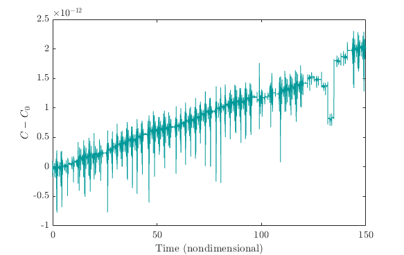
As can be seen on that figure, the Jacobi constant is constant up to the 11th digit after the decimal point. This accuracy is quite reasonable for that kind of problem but if a higher accuracy is required, the relative tolerance and/or the absolute tolerance could be reduced.