Kepler Orbit

Problem Definition

For this example, we consider a spacecraft on a Kepler orbit about the Earth and we want to predict its future trajectory. We assume that the elliptical orbit is described by the following classical orbital elements:

• Semi-major axis: a = 20,000 km
• Eccentricity: e = 0.7
• Inclination: i = 35°
• Right ascension of the ascending node: Ω = 100°
• Argument of perigee: ω = 65°
• True anomaly: ν = 30°

The period of an orbit is given by $P = 2\pi\sqrt{\frac{a^3}{\mu}}$ where $\mu$ is the standard gravitational parameter. For the Earth, μ = 398600.4354 km³/s² and thus P = 2.8149 $\cdot$ 10⁴ s = 7.82 hours. The initial position of the spacecraft expressed in Cartesian coordinates is

$$\mathbf{r} = \begin{bmatrix} -5007.2484 & -1444.9181 & 3628.5346 \end{bmatrix} \quad km$$

and velocity

$$\mathbf{v} = \begin{bmatrix} 0.7177 & -10.2241 & 0.7482 \end{bmatrix} \quad km/s$$

such that the initial state vector is $\mathbf{s} = [\mathbf{r}, \mathbf{v}]^{T}$. The equations of motion describing the evolution of the system are

$$\ddot{\mathbf{r}} = -\frac{\mu}{r^3}\mathbf{r}$$

where $r$ is the magnitude of $\mathbf{r}$. Since the crate handles first order ODEs, this system must be transformed into a state space form representation. An appropriate change of variables $y_1 = r_1$, $y_2 = r_2$, $y_3 = r_3$, $y_4 = \dot{r}_1 = v_1$, $y_5 = \dot{r}_2 = v_2$, $y_6 = \dot{r}_3 = v_3$ yields

$$\dot{y}_1 = y_4$$

$$\dot{y}_2 = y_5$$

$$\dot{y}_3 = y_6$$

$$\dot{y}_4 = -\frac{\mu}{r^3}y_1$$

$$\dot{y}_5 = -\frac{\mu}{r^3}y_2$$

$$\dot{y}_6 = -\frac{\mu}{r^3}y_3$$

which can be numerically integrated.

Implementation

The problem is solved using the Dopri5 method. We first import the crate and bring the required modules into scope:

use ode_solvers::dopri5::*;
use ode_solvers::*;

Next, two type aliases are defined:

type State = Vector6<f64>;
type Time = f64;

and a structure containing the parameters of the model is created:

struct KeplerOrbit {
  mu: f64,
}

The System<V> trait is then implemented for KeplerOrbit:

impl ode_solvers::System<State> for KeplerOrbit {
    // Equations of motion of the system
    fn system(&self, _t: Time, y: &State, dy: &mut State) {
        let r = (y[0] * y[0] + y[1] * y[1] + y[2] * y[2]).sqrt();

        dy[0] = y[3];
        dy[1] = y[4];
        dy[2] = y[5];
        dy[3] = - self.mu * y[0] / r.powi(3);
        dy[4] = - self.mu * y[1] / r.powi(3);
        dy[5] = - self.mu * y[2] / r.powi(3);
    }
}

We now implement the main function. The system of ODEs is first created with the corresponding $\mu$ parameter. The orbital period is then computed and the initial state is initialized. The integration will be carried out using the 5th order Dormand-Prince method. Hence, a Dopri5 structure is created with the system structure, the initial time, the final time, the time increment between two outputs, the initial state vector, the relative tolerance, and the absolute tolerance as arguments. The integration is launched by calling the method integrate() and the result is stored in res. Finally, a check on the outcome of the integration is performed and the outputs can be extracted.

fn main() {
    let system = KeplerOrbit {mu: 398600.435436}

    let a: f64 = 20000.0;
    let period = 2.0 * PI * (a.powi(3) / system.mu).sqrt();
    let y0 = State::new(-5007.248417988539, -1444.918140151374, 3628.534606178356, 0.717716656891, -10.224093784269, 0.748229399696);

    let mut stepper = Dopri5::new(system, 0.0, 5.0 * period, 60.0, y0, 1.0e-10, 1.0e-10);
    let res = stepper.integrate();

    // Handle result
    match res {
        Ok(stats) => {
            stats.print();

            // Do something with the output...
            // let path = Path::new("./outputs/kepler_orbit_dopri5.dat"); 
            // save(stepper.x_out(), stepper.y_out(), path);  
            // println!("Results saved in: {:?}", path);
        },
        Err(_) => println!("An error occured."),
    }
}

Results

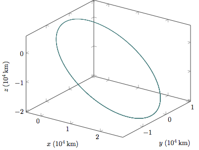
The following figure shows the trajectory resulting from the integration. As expected, the orbit is closed.

Some information on the integration process is provided in the stats variable:

Number of function evaluations: 62835
Number of accepted steps: 10467
Number of rejected steps: 5

In order to assess the accuracy of the integration, we look at the specific orbital energy which is a constant of the motion. This specific energy is given by

$$\varepsilon = \frac{v^2}{2} - \frac{\mu}{r}$$ where $v$ is the amplitude of the velocity and $r$ is the distance from the Earth's center to the spacecraft. In theory, this value is constant as long as no external force acts on the system (which is the case here). From the intial conditions, the specific energy of this orbit is $$\varepsilon_0 = -9.9650 \; km^2/s^2$$ By computing $\varepsilon$ for each time step and plotting the difference $\varepsilon_i - \varepsilon_0$, we obtain the following time evolution of the error:

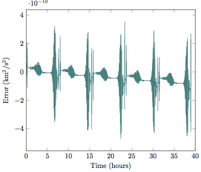
As can be seen on this figure, the specific energy is constant up to the 9th digit after the decimal point which shows that the accuracy of the integration is quite good. A higher accuracy can be achieved by selecting smaller values for rtol and atol.